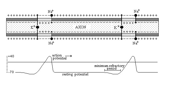
Figure 5.1. The axon and the action potentials.
This chapter discuss:
More than fifty years ago action potentials were first recorded by means of external electrodes by Hodgkin and Huxley (1939). Based on the results of their experiments they designed a new revolutionary theory about action potential generation which meant a breakthrough in electrophysiology at the time.
In 1952 Hodgkin and Huxley published a quantitative model of the electrical and electrochemical phenomena in the environment of the membrane of a nerve fiber based on their theory. The original model of Hodgkin and Huxley was not a mathematical model but an electric circuit consisting of capacitors and resistors. however, it is very simple to transfer this model into a mathematical model. The prototype AXON is based on such a mathematical model.
Educational value
Although some of the aspects of the conductivity of the cell membrane were not described correctly by Hodgkin and Huxley, their model is still very useful for the education of medical students and biology students as it can be used as a simplified version of the correct model thus helping the students to build a conceptual 'framework' model which can be filled with the complete and correct conceptual model in a later phase of their education.

It can also be used as a demonstration for the experimental research techniques used in cell physiology. Furthermore, the model can be used for biology courses in secondary education, as the differences between the results of the model of Hodgkin and Huxley and the real cell membrane system are not relevant at this level.
Model description
When the membrane of a nerve fiber is simulated an action potential may be generated depending on the polarization of the membrane. After the generation of an 'action potential' the membrane becomes hyperpolarized for some time, depending on the intensity of the stimulus. For this reason a higher intensity or the right moment in time is required for a second stimulus in order to generate a second action potential (see figure 5.1, 5.2 and 5.3). The program AXON was designed by Scholten & Verhoeven (1987) in order to enable students to experiment with a nerve cell system. Students are able to stimulate the nerve cell twice and to study the resulting phenomena. The starting values of the model are:
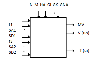
The default values of the parameters are:
The most essential parts of the model written in Pascal are:
The program is designed according to the description of the students' learning environment of MacTHESIS. In this application two windows are present:

Students may intervene with the model by means of the input-animation technique as described above. Furthermore the same interventions (start of the first stimulus, duration of the first stimulus, intensity of the first stimulus, start of the second stimulus, duration of the second stimulus, intensity of the second stimulus) are possible by means of the menu bar.
The prototype CHEMISTRY simulates titration experiments. The titration of acid solutions by means of bases can be simulated as well as the titration of basic solutions by means of acids. The simulation of strong acids and bases is possible as well as the simulation of weak acids and bases. The model on which CHEMISTRY is based has been derived by van Schaick Zillesen and Min from general theories about acid-base equilibria.
Educational value
CHEMISTRY is designed in order to enable students to practice the skill to determine the properties (strength, pKa, pKb) of solutions of acids and bases by titration with standardized acids or bases. Furthermore, students may use the program to exercise two skills:
- the skill to calculate the pH of a solution of which the original composition is known after the addition of known quantities of standardized solutions (acids, bases or water).
- the skill to recalculate the original composition of a solution of which the pH and the quantities of standardized solutions added to it are
known.
The simulated experiments can be executed very accurately because drops
of acid or base can be added to the solution one after another. The speed of the chemical reactions is retarded in the simulation. For this reason
it may take some time before the reaction caused by the addition of a drop of acid or base is completed. This dynamic aspect may facilitate the discrimination
of the chemical reactions causing the observed phenomena.
Furthermore, time registrations of the pH, the pOH, the concentration
of cation of base, the concentration of anion of acid, the concentration of non-ionized
base and the concentration of non-ionized acid are provided for in the simulation.
In a real laboratory this complete information can only be attained by means
of expensive ion-sensitive electrodes.
Boblick (1971) emphasized that students may use computer simulations of titration experiments to demonstrate their achievements in a faster, safer and more efficient way. He also asserted that the method of computer simulation eliminates the necessity to acquire a number of psychomotor skills in order to demonstrate the achievement of intellectual skills. Nowadays chemists seldom perform a titration manually in the way it is taught in secondary education. The invention of advanced electronic instruments (pH meters and automatic burettes) have made the psychomotor skills acquired during secondary education, obsolete for everyday chemical applications. For this reason Boblick (1971) states that the acid-base titration during secondary chemistry teaching can no longer be important as a laboratory technique, but as a means of demonstrating the application of chemical principles. This statement implies that it is best to put the emphasis on the acquisition of intellectual skills and not on the acquisition of psychomotor skills when teaching titration during secondary education. Compared with real titration experiments computer simulations executed with programs like CHEMISTRY may be more suitable to gain the required intellectual skills because of the advantages mentioned above.
Implementation
The MacTHESlS version of CHEMISTRY was implemented by Van Schaick Zillesen in order to test the suitability of the MacTHESlS system for designing simulations of laboratory equipment.
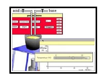
In this application three windows are present (See figure 5.5):
- In the first window the experimental apparatus is visualized.
The apparatus consists of three burettes filled with acid, water and base and a flask containing an unknown solution. The pH and the pOH in the flask
are indicated in this window. In the taps of the burettes black dots are present. Students may control the opening of the taps of the burettes by means of direct manipulation conform the input-animation technique.
- The second window contains time registrations of the pH and the pOH in the solution.
- The third window contains time registrations of the logarithms of the concentrations of anion of Acid, cation of Base, non-ionized Acid and non-ionized Base.
Students may intervene with the model by means of the input-animation technique as described above. Furthermore, the same interventions are possible
by means of the menu-bar.
At the start of the program the flask contains pure water. However, a student can select other solutions by means of the menu-bar by activating
the option 'case'. The following solutions are provided for:
- a solution of a strong base
- a solution of a strong acid
- a solution of a weak acid
- a solution of a weak base
Model description
In the simplest part of the model of a titration, are these two basic equations:
dH3O/dt = - k1*H3O*OH + k2*H2O*H2O
dOH/dt = - k1*H3O*OH + k2*H2O*H2O
in which 0.1 mol reacts with 0.1 mol NaOH, we assume that there is in the water (constantly 1 liter) a balance of 10-7 mol H3O+ and OH-, and 55.6 mol H2O.
The starting values of the model are:
The default values of the parameters are:
tap = 0
k1 = 0.1
k2 = 0
k3 = 0
k4 = 0.1
k5 = 100
k6 = 1.0E-14 * k5 / (H2O*H2O)
vol = 0.5
voloud = vol
volb = 0.1
volp = 0.02
molz = 0.1
molb = 0.1
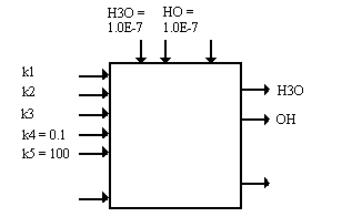
The most essential part of the model in Pascal is:
H3Ooud := H3O;
OHoud := OH;
H3O := H3Ooud + dH3Odt*dt;
OH := OHoud + dOHdt*dt;
vol := voloud + dthulp / dt * (vol - voloud);
H2O := H2O + dH2Odt * dthulp;
HCl := HCL + dHCldt * dthulp;
Cl := Cl + dCldt * dthulp;
NaOH:= NaOH + dNaOHdt * dthulp;
Na := Na + dNadt * dthulp;
t := t + dthulp;
pH := - ln(H3O) / ln(10);
pOH := - ln(OH) / ln(10);
Until t > Tmax; (* 40 *)
The procedures Zuur, Base, Verdun and Pasaan are described in the appendix. The variables ZuurinBuret and no ZuurinBuret and these procedures are necessary for input possibilities in case of titration, specially if there is not a steady state in the solution.
Educational value
LEMMING has been designed in order to enable students in secondary education to experiment with a simulated relatively simple ecosystem. By means of active experimentation students may experience the mutual dependency
of the main biotic components of the ecosystem: plants, herbivores, carnivores and decomposers. Furthermore they may experience the role of abiotic factors
(like the climate and the availability of nutrients) in the system.
Implementation
The MacTHESlS version of LEMMING is constructed to be used as an example
for a simulation of a predator prey relation. The educational goals were similar to those described for the prototype FOOD CHAIN. The prototype was designed for the same population of students (lower secondary education). However, when the two prototypes were
compared, the suitability of the prototype FOOD CHAIN for this population of students proved to be better, since more relatively simple experiments could be executed by means of this prototype. The experiments which could be executed by
means of LEMMING were generally too difficult for this group of students.
Therefore the further development of this prototype was ceased.
Model description
The prototype LEMMING, version MacTHESlS, has been designed according to the description of the learning environment of MacTHESlS:
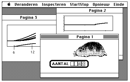
- In the first window the main components of the ecosystem are drawn. The present values of the main variables in the system are indicated by means of dynamic decimal numbers (number of lemmings and number of arctic
foxes).
Students may intervene in the model by changing its most relevant parameters (biomass of food, number of lemmings, number of arctic foxes, litter size of lemmings and litter size of arctic foxes) by clicking in the buttons
drawn underneath the drawings, in conformity with the input-animation technique.
- The second window contains a time registration of the biomass of food, the number of lemmings and the number of arctic foxes.
- The third window contains a dynamic histogram showing the present values of the same variables as displayed in the second window. The differences between the phases of the fluctuations of the variables can be clearly observed in this window.
Students may select one of the following cases using the menu-bar:
- An ecosystem with herbs only
- An ecosystem with herbs and lemmings
- An ecosystem with herbs, lemmings and arctic foxes
- An ecosystem with herbs, lemmings and arctic foxes in a relatively cold climate
The default values of the parameters are:
Some boundaries, maximum and minimum are:
MIP = 0.17
MP= 0.55
RMI = 5
RMA = 120
PTMAX = 4
The starting values of the model are:
PRO = 50
RO= 0
VDSL = VB0 * KB
CP= MIP
VB= VB0
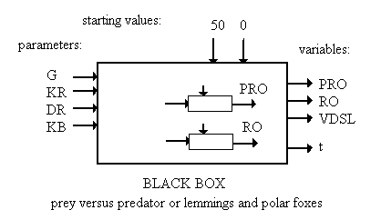
The most essential parts of the model written in Pascal are:
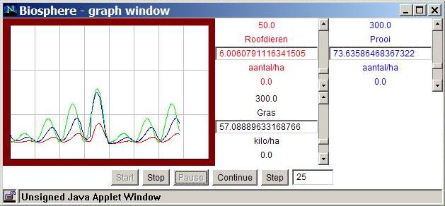
About the classic predator or prey model much has been said in chapter 1, figure 1.4 and 1.5. In figure 5.7 the variables fluctuate periodically (oscilate).
When this phenomena will be showed in a x-y plane (phase plane) a 'limit cycle' can be seen: the population set out along the x-axis fluctuates between two values and the population set out along the y-axis also fluctuates between two values. This phenomena of a limit cycle is an indication that the model oscillates. A normal time diagram y=f(t) shows in that situation that the variables fluctuate between two values along the y-axis.
Many mathematical models of a RC network can be designed and realized. This model describes a low frequency filter and a high frequency filter. The models can be used in order to study the network behaviour in a dynamic way by changing the resistances and the capacities in relation to the input and output voltages (see figure 5.9).
The model has been implemented in the prototype RC NETWORK, built with MacTHESIS. The model has been developed for educational applications.
Educational value
Simulations of electronic networks may be useful in the curriculum of physics and electro-technics to replace real experiments. However, the
aim of the design of the described prototype was not the implementation in an existing curriculum, but a test of the suitability of the design
method for the implementation of mathematical models originating from the subject of electronics.
Model description
The prototype RC NETWORK is designed according to the description of
the student's environment of MacTHESlS. The essential parts of the model are the starting values, the default parameter values and de mathematical model in Pascal.
The default values of the parameters are:
switch1 = 0; <- 0 or 1
switch2 = 0; <- 0 or 1
switch3 = 0; <- 0 or 1
T1= 0;
A=8
f=2;
s=1;
R1=0.1; R2=0.1;
C1=0.3; C2=0.3;
The starting values of the model variables are:
ui1= 0.0; ui2 = 0.0; ui3 = 0.0;
u1 = 0.0; u2 = 0.0; uh = 0.0;
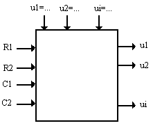
The most essential parts of the model written in Pascal are:
Repeat
ui1 := switch1*A*sin(2*3.14*f*t);
ui2 := switch2*A*sin(2*3.14*f*t) / abs(sin(2* 3.14*f*t));
if t > T1 then ui3 := switch3*A else ui3:= 0.0;
ui := ui1 + ui2 + ui3;
i1 := (ui - u1) / R1; <- Filter 1
du1dt := i1 / C1;
u1 := u1 + du1dt*dt;
i2 := u2 / R2; <- Filter 2
duhdt := i2 / C2;
uh := uh + duhdt*dt;
u2 := ui - uh;
Until t > Tmax
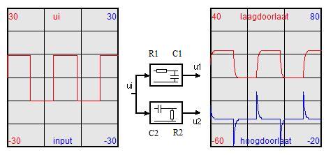
In the screendump of the 'RC filter' application in figure 5.10, two graphical viewports are presented and a conceptual model of the filter with R1, C1, R2 and C2.
In the middle a diagram of the simulated electronic circuit is visualized. The circuit consists of two networks of a resistor and a capacity and a (hiden) function generator. Students can change the form (sinus, block or pulse), frequency (f) and amplitude (A) of the input by clicking in the buttons on the function generator, in conformity with the input-animation techniques of this software. The properties of the electronic network can be changed by clicking in one or more resistor(s) (R1 or R2) or capacity(ies) (C1 or C2). In the two dynamical 'growing' graphs 3 time registrations are displayed: the input (ui) and the output variables (u1 and u2) [volt].
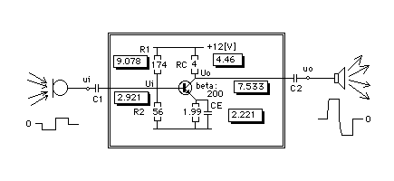
Many mathematical models of a transistor are known. Some of these models are matrix-models, treating the transistor as a black box, presenting sets of values of output variables as a result of sets of values of input parameters like input impedance, voltage gain etc. Other models simulate the transistor in a more transparent way. In these models, the transistor is described by means of an electronic circuit. The models can be used in order to study the transistor's behaviour in a dynamic way by changing the parameters.
The model of a transistor, implemented in the prototype TRANSISTOR, belongs to the second type of models. It describes the behaviour of a transistor in a normal low signal amplifier circuit. The model has been developed for educational applications by Min and Malhotra (1988) and Min and Van Leeuwen (1990, not published) (see figure 5.11).
Educational value
Simulations of electronic networks may be useful in the physics or electronics curriculum as a training before starting real experiments.
The consultation of content specialists, curriculum specialists and specialists in didactics would be required in order to obtain the information needed
for the improvement of the prototype in order to make it suitable for use in a didactic environment.
Nevertheless, prototypes similar to TRANSISTOR may prove very useful in everyday physics teaching to replace expensive or difficult experiments.
Model description
TRANSISTOR has been first implemented in MacTHESlS by Malhotra in 1988.
The purpose of the implementation was to test the performance of the design system with respect to the implementation of models originating from the subject of Physics. Min and Van Leeuwen have implemented TRANSISTOR in MacTHESIS in 1990.
The default values of the parameters and the starting values of his model are:
A = 0.01
<- V
f = 100.0 <- Hz
ui = 0.0
<- V
beta = 200.0
IC0 = 1.0 <- mA
q = 1.6E-19 <- Asec
K = 1.38E-23 <- J/K
T = 100.0 <- K
S = 40.0*IC0 <- (q / K.T).IC0
= 40.0
rb = beta/S <- 5 kOhm
Ucc = 12.0 <- V
IB0 = IC0/beta <- 1/200=0.005
mA
IE0 = (beta + 1)*IB0 <- (200+1)0.05
= 1.005 mA
RC = 4.0 <- kOhm
R2 = 56.0 <- kOhm
RE = (0.5*Ucc - IC0*RC)/IE0 <- 2/1.005 kOhm
Ir = (0.7 + RE*IE0)/R2 <- 2.71/56 = 0.04839 mA
R1 = (Ucc-0.7-RE*IE0)/(IB0+Ir) <-
174.0 kOhm
ib = ui*S/beta
uo = -beta*ib*RC
The most essential parts of the model written in Pascal are:
Repeat
t := t + dt;
ui := A * sin (2 * 3.1418 * f * t);
S := 40 * IC0;
IB0 := IC0 / beta;
IE0 := (beta+1) * IB0;
RE := (0.5*Ucc - IC0*RC) / IE0;
Ir := (0.7 + RE*IE0)/R2;
R1 := (Ucc - 0.7 - RE*IE0) / (IB0 + Ir);
i1:=ui/R1;
i2:=ui/R2;
ib := ui * S / beta;
ii := i1+i2+ib;
uo := -beta*ib*RC;
io :=uo/RC;
Until t > Tmax;
The prototype TRANSISTOR is designed according to the description of the student's environment of MacTHESlS:
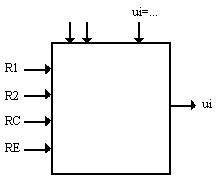
In the first window a diagram of the simulated electronic circuit is visualized. The circuit consists a 'standard' transistor, some resistors and a function generator. Students can change the form (sinus, block or pulse), frequency and amplitude of the input voltage on the circuit by clicking in the buttons on the function generator, in conformity with the input-animation techniques of MacTHESIS software.
The prototype TRANSISTOR is first designed according to the description of the student's environment of MacTHESlS. In this application 3 windows are present. In other versions mostly two window are visualized. The circuit consists a 'standard' transistor, some resistors and a function generator.
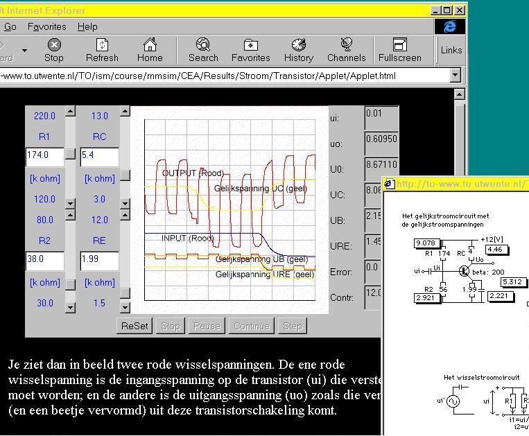
The properties of the electronic network can be changed by clicking in one of the resistors or some part of the transistor.
Note
Most paragraphs of this chapter have been written by P.G. van Schaick Zillesen (edited by F.B.M. Min) and first versions were published in the thesis of Van Schaick Zillesen, University of Twente, Enschede (1990).
Gerestaureerd in 2020