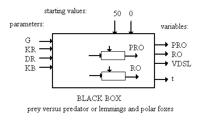
Figure 1. The classical famous prey-beast-predator model from the biology; here: the 'struggle' between lemmings (NB or PRO, prooi of buit) versus polar foxes (NR or RO, roofdier).
After an outbreak of lemmings it will usually take three or four years before the next outbreak occurs. Fluctuations of predators like arctic foxes, which are dependent on lemmings as their main source of food, usually show the same pattern as the lemming fluctuations (with some delay).
Schultz (1969) described the relations between lemmings, their food (herbs), their predators (mainly arctic foxes) and the bottom of the arctic tundra. He emphasized the role of changing nutrient concentrations in the dynamics of the arctic tundra system. In the spring of a year with an outbreak of lemmings almost all minerals are present in the herbs. However, as a result of the consumption by the rodents most of these nutrients are deposited on the surface of the tundra in the form of faeces during the same year. The next year plant growth is minimal because of the low nutrient concentrations prevailing in the soil. It will take several years for the faeces to mineralize because of the extreme polar climate. However, the third year after the outbreak the mineral level of the tundra soil has gradually increased to a point that enables rapid plant growth. However, the nutrient level in the crop is still very low during this year. A high nutrient level in the crop, enabling a good lactation in lemming females, is required in order to cause a lemming breeding success. For this reason the number of lemmings does not rise proportionally to the plant growth during this year. However, during the next year the nutrient concentration in the herbs is much higher causing a new outbreak of lemmings (see figure 1 and 2).

The program LEMMINGS simulates the processes described above. The model on which the program is based has been developed as part of this study and has so far not been published anywhere else.
Educational value
LEMMINGS has been designed in order to enable students in secondary education to experiment with a simulated relatively simple ecosystem. By means of active experimentation students may experience the mutual dependency of the main biotic components of the ecosystem: plants, herbivores, carnivores and decomposers. Furthermore they may experience the role of abiotic factors (like the climate and the availability of nutrients) in the system.
Implementation
The MacTHESlS version of LEMMINGS is constructed to be used as an example for a simulation of a predator prey relation. The educational goals were similar to those described for the prototype FOOD CHAIN. The prototype was designed for the same population of students (lower secondary education). However, when the two prototypes were compared, the suitability of the prototype FOOD CHAIN for this population of students proved to be better, since more relatively simple experiments could be executed by means of this prototype. The experiments which could be executed by means of LEMMINGS were generally too difficult for this group of students. Therefore the further development of this prototype was ceased.

Model description
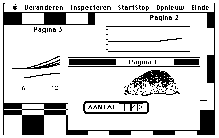
The prototype LEMMINGS, version MacTHESlS, has been designed according to the description of the learning environment of MacTHESlS. In this application three windows are present (presented in figure 3):
Students may select one of the following cases using the menu-bar:
The default values of the parameters are:
KB= 170
VB0 = 30 / KB
CPKR = 0.48
G = 16
R = 5
KR= 2
DR= 0.05
S = 20 * DR
Some boundaries, maximum and minimum are:
MIP  = 0.17
MP= 0.55
RMI   = 5
RMA  = 120
PTMAX  = 4
The starting values of the model are:
PRO = 50 (startwaarden prooidieren)
RO= 5 (or 0) (startwaarden roofdieren)
VDSL = VB0 * KB
CP= MIP
VB= VB0
The most essential parts of the model written in Pascal are:
Repeat
  CP   := CP + ((MP - MIP) / PTMAX) * dt;
  VB   := VB0 + (CP - MIP) * (1 - VB0) / (MP - MIP) * (1 - COS(t  * CRCL)) / 2;
  VDSL := VB * KB;
  RO  := RO + (G * RO * (KR - RO + DR * PRO) / (KR+DR*PRO)) * dt;
  PRO  := PRO + (R * PRO * (VDSL - PRO - S * RO) / VDSL) * dt;
Until t > Tmax;     (* 4 years  *)
About the classic predator or prey model much has been said by others.

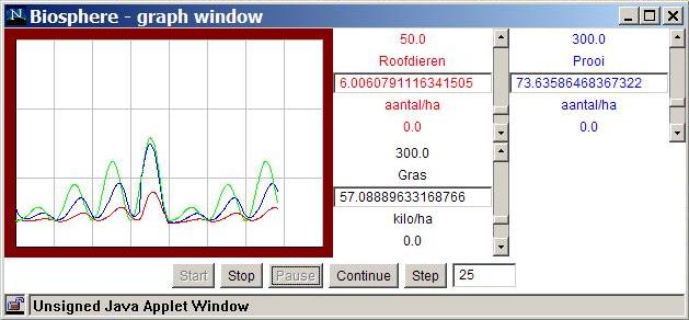
In figure 4 the variables fluctuate periodically (oscilate). When this phenomena will be showed in a x-y plane (phase plane) a 'limit cycle' can be seen: the population set out along the x-axis fluctuates between two values and the population set out along the y-axis also fluctuates between two values. This phenomena of a limit cycle is an indication that the model oscillates. A normal time diagram y=f(t) shows in that situation that the variables fluctuate between two values along the y-axis.

Rik Min, Enschede, March, 2003; updated 2005. Gerestaureerd in 2020.